From the previous episode…

In a previous post, we have talked of a recent paper that was investigating the locality of NL-means. This paper by Simon Postec pointed out the following paradox:

The more NL-means is nonlocal, the less it is a good denoising algorithm.

Indeed, this phenomenon was seldom observed and even less investigated, since for computational reasons most NL-means (and derivatives) are experimented with small learning neighbourhoods only. So, shall we consider that NL-means is local after all?

Experimental confirmation

In this post, we will confirm experimentally the results from Postec et al.

I will also take advantage of the post to present an implementation of NL-means in Python, because:

• I want to learn and practice Python, and that’s a good reason per se!
• I didn’t find any code from Simon Postec or his co-authors, so let’s make a bit of Reproducible Research¹.

So, let’s dive into the code!

A Python implementation of NL-means

Extracting patches

NL-means is a patch-oriented processor. Obviously, we’ll need a patch extractor. Here is a simple one, that applies mirroring on the image boundaries:

def extract_patch_at_location(location, image, patch_half_size, patch_length=None):

    """Compute a row vector for the patch at location (x,y)=(col,row)."""
    (height, width) = image.shape

    if patch_length is None:
        patch_length = (2*patch_half_size+1)*(2*patch_half_size+1)
    patch = np.zeros((1, patch_length))

    dest = 0
    for j in range(-patch_half_size, patch_half_size+1):

        y = location[1]+j
        # Boundary check                                                                                                                                                                                   
        if y < 0 or y >= height:
            y = location[1]-j

        for i in range(-patch_half_size, patch_half_size+1):

            x = location[0]+i
            # Boundary check                                                                                                                                                                               
            if x < 0 or x >= width:
                x = location[0]-i

            patch[0, dest] = image[y, x]
            dest = dest+1

    return patch

My personal style for implementing NL-means is a bit unusual: I collect all the patches first and I store them in a matrix. Regular implementations usually build the patches on the fly. Building the patches on the fly has some advantages on lower-memory devices², but nowadays RAM is cheap and building the patches first allows for easier parallel processing later.

Comparing the patches

Once we have patches, NL-means will denoise each pixel by comparing the corresponding patch with the patches of all the pixels in a learning neigbourhood centered on this pixel. The denoised value will be the weighted average of all these pixels, where the weights are given by the formula:

$$w(P(\mathbf{x}), P(\mathbf{y})) = \frac{1}{Z} \exp \left( - \frac{| P(\mathbf{x}) - P(\mathbf{y}) |_2^2}{h^2} \right).$$

$P(\mathbf{x}), P(\mathbf{y})$ are the two patches to be compared, $h$ is a filtering parameter, and $Z$ a normalization constant (the sum of all the weights in the learning neighbourhood).

For simplicity, I have omitted the multiplication of teh patches by a Gaussian window (that has for effect to emphasize the center part of the patch), but in practice this yields only slightly different results.

The only difficulty is how to deal with the central pixel. In the weight formula, the central pixel will always have a weight of 1 and will reduce the efficeincy of the denoising. Thus, I will not compute a weight for this particular location, but will assign it the maximum of the weights computed inside the learning window.

# Learn a denoised patch value in a neighbourhood
def explore_neighborhood_greedy(pixel, learning_neighborhood, patches, noisy_image, h2, patch_distance=l2sqr):

    """Compute the weights and sme statistics around a given pixel."""
    (l_min, l_max) = learning_neighborhood
    (h, w) = noisy_image.shape

    sum_w = 0.0
    max_w = 0.0
    weighted_sum = 0.0

    reference = pixel[0]*w + pixel[1]

    for (y, x) in it.product(xrange(l_min[0], l_max[0]), xrange(l_min[1], l_max[1])):
        if y is not pixel[0] or x is not pixel[1]:
            patch = y*w + x

            w = patch_distance(patches[reference, : ], patches[patch, : ])
            w = w**2 / h2
            w = exp(-w)

            weighted_sum = weighted_sum + w*noisy_image[y, x]
            sum_w = sum_w + w
            max_w = max(w, max_w)

    return weighted_sum, sum_w, max_w

Getting the final denoised value

The denoised value for the pixel at hand is obtained by taking the weighted sum of all the pixels in the learning window, adding the value of the central pixel (multiplied by the maximum weight in the neighbourhood) and dividing by the sum of the weights. In other words, a barycenter.

# Apply NL-means to an image
def nlmeans_basic(noisy_image, noisy_patches, learning_window_half_size, h,
                  explore_neighborhood_fn=explore_neighborhood_greedy):

    """Apply the NL-means procedure to an image given some patches."""
    (rows, cols) = noisy_image.shape
    h2 = h*h

    clean_image = np.zeros_like(noisy_image)

    # Main denoising loop                                                                                                                                                                                  
    for (y, x) in it.product(xrange(0, rows), xrange(0, cols)):

        # Learning neighbourhood exploration                                                                                                                                                               
        learning_min = (max(0, y-learning_window_half_size), max(0, x-learning_window_half_size))
        learning_max = (min(rows, y+learning_window_half_size), min(cols, x+learning_window_half_size))
        out_grey, sum_weight, max_weight = explore_neighborhood_fn((y, x), (learning_min, learning_max), noisy_patches, noisy_image, h2)

        # Central pix handling                                                                                                                                                                             
        if sum_weight > 1e-6:
            sum_weight = sum_weight + max_weight
            out_grey = out_grey + max_weight*noisy_image[y, x]
            out_grey = out_grey / sum_weight
        else:
            out_grey = noisy_image[y, x]

        # Now, write the denoised output                                                                                                                                                                   
        clean_image[y, x] = out_grey

    return clean_image

Et voilà !

The final routine is really simple: computing the bounds of the learning windows, computing the weights, assigning the barycenter as output. And this is probably the most stunning part of NL-means: its simplicity.

Experimental results

I’ve added a Gaussian noise of standard deviation 0.2 times the dynamic range to an image of Lena³. Then, I’ve fixed the value of the $h$ parameter to 2 and run NL-means for two different patch sizes: $5 \times 5$ and $7 \times 7$ pixels. Finally, for each patch size I let the learning neighbourhood size vary from $3 \times 3$ to $21 \times 21$.

The following figure shows the MSE for each patch and learning neighbourhood size. The neighbourhood size 0 depicts the original noisy image, and the horizontal axis depicts the half learning neighbourhood size. The final learning neighbourhood size is given by twice this value plus 1.

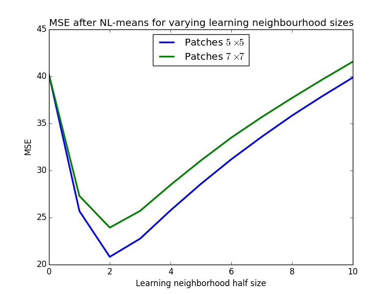
As can be seen from the graph, both patch sizes exhibit the same phenomenon: when the learning neighbourhood gets bigger than $5 \times 5$ pixels, the denoising performance starts to decrease. This is slightly worse than the result in Postec et al., but this can be due to the lack of a Gaussian window, a bad choice of $h$ or simply by chance since I used only 1 test image and 1 noise pattern.

Conclusions and future post

In this post, we have seen an example of an easy, non-optimized implementation of NL-means. Using this implementation, we have been able to confirm the observations from the Postec et al. paper: NL-means efficiency is reduced when the implementation gets more non-local!

Show me the code!

I plan to release the full code package when the post series is complete. I would like to make another two or three posts⁴.

Next post

In the next post, I will make a small experiment to confirm Postec’s intuition about the locality of NL-means: the nonlocal hypothesis is more easily violated far from the pixel to be denoised.