Non-locality and NL-Means
Non-locality is a powerful recent paradigm in Image Processing that was introduced around 2005. Put in simple words, it consists in considering that an image is a collection of highly redundant patches. In this context, pixels get described by the surrounding patch instead of their sole value), and patch relationships are only deduced from their visual similarity (thus ignoring their spatial relationship).
Non-locality comes in two flavors: exemplar-based 1 or sparsity-based. The most famous example of sparsity based non-local algorithm is BM3D, and it is still considered as a top-ranking denoising algorithm.
In this series we are interested in the very popular Non-Local means, that are inspired from exemplar-based algorithms. NL-Means are conceptually much simpler than BM3D, yet is still a very powerful denoising method. Hence, they are a very good introduction to the non-local intuition.
NL-means did also inspire a lot of derivative work.
The NL-Means algorithm
The intuition
There is one big secret behind NL-means denoising:
Denoising is as simple as averaging.
The real problem is: what should be averaged ?
Averaging spatially connected yields blur, so it is not a good solution. Luckily, here comes non-locality!
There exists a well known and very simple denoising method: averaging. However, it is also well known that averaging pixels in an image yields a lot of undesirable blur that destroys both the noise and the texture of the image.
The reason for this is simple: pixels can’t be assumed to be measurements of the same static phenomenon just because they are spatially close inside the image! For example, this assumption will be violated along the edges of each object, or everywhere a light or color gradient exists.
The NL-means algorithm
To avoid this undesirable blur, NL-means forgets about spatial relationship between pixels. This is why it is called a non-local algorithm.
Instead of using spatial coordinates, we are left with their color (or gray level). Since considering only a single pixel value is error prone2, we zoom out a bit to consider a small square around the pixel of interest. This small square is called a patch.
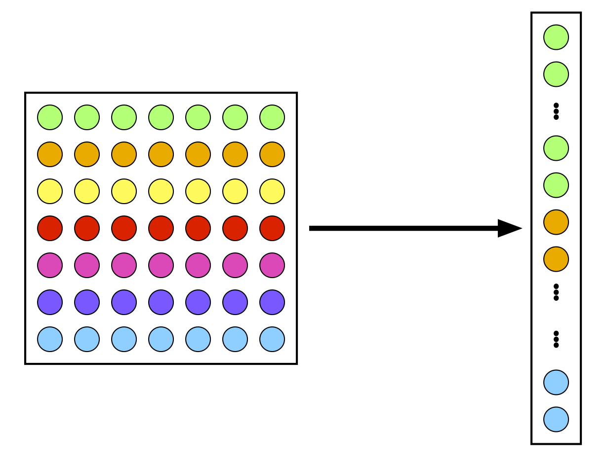
A patch is transformed into a feature vector simply by reshaping it as a vector. It can also be interpreted as the coordinates of the central pixel in a high dimensional space that describes all the possible image patches.
Then, instead of using spatial proximity between pixels, the distance between their patches is computed. The denoised value of a given pixel is obtained as the weighted average of the other pixels of the image, where the weight (or contribution) of each pixel is inversely proportional to the distance between its patch and the reference patch of the pixel to denoise.
Next posts
In the next post, I will introduce the mathematical formulation of NL-means. Then, we will see typical implementations.
Once we have a good understanding of NL-means, we will come to the real novelty:
- a simple experiment that shows that choosing a very nonlocal NL-means implementation can yield worse results than a local one!
- some simple strategies to speed-up the computations while retaining the main qualities of the original NL-means.
So stay tuned!
If you don’t want to miss the next post, you can register to the blog’s feed or follow me on Twitter !