In the previous episode, we have seen the main idea of NL-means:
A good denoising algorithm can be obtained by a simple weighted average of noisy pixels, at the condition that the weights depend on the content of patches around the pixels instead of their spatial distance.
In this post, we will put proper mathematical definitions behind those patches and weighted average. I will proceed in successive steps:
- first define what a digital image, and consequently the patches as subparts of the images
- then introduce a distance between patches, such that small distance values correspond to identical patches and large values to dissimilar patches
- then, computing weights from these distances that can be used in a denoising process
- and finally, how to obtain denoised pixel values.
So, let’s dive in!
Mathematical framework
$\def\x{\bf x}\def\y{\bf y}\def\G{\mathcal{G}} \def\RR{\mathbb{R}} \def\R{\bf R}$
Digital images and patches
From now on, we suppose that we are given an image \(I\) defined on a domain \( \Omega \subset \RR^2 \), The image has values in $\RR$ (for grayscale images) or $\RR^3$ (for color images). We write $\x,\y \in \Omega \times \Omega$ two pixel locations. We define a patch extraction operator $\R$ that returns the pixels inside a squared $\sqrt{d} \times \sqrt{d}$ neighbourhood around $\x$ and stacks them in a vector using lexicographic ordering:
$$\R : \x \mapsto \R(\x) = ( I(x_1), \ldots, I(x_d) )^T \in \RR^d.$$
Distance between patches
Given two patches, we define the distance between them as the usual squared Euclidean distance:
$$ d \left( \R(\x), \R(\y) \right) = | \R(\x) - \R(\y)|_2^2 = \sum_{i=1}^d \left( \R(\x)_i - \R(\y)_i \right)^2. $$
Weights (or similarity score)
Given the distance between two patches, one can compute their visual similarity, normalized into the interval $ [0,1] $ (ranging from no similarity to identical) by a simple exponential filtering:
$$ w(\x,\y) = \exp { {-\frac{d(\x,\y)}{h^2} } } = \exp { - \frac{| \R(\x) - \R(\y) |^2_2}{h^2} }. \label{eq:nl-w} $$
The values of $w(\x,\y)$ are obviously between 0 and 1. The parameter $h$ controls the decay of the exponential function: for small $h$, only very similar patches will have a significant similarity score and the filter will be very selective. On the other hand, a large $h$ will attribute a more uniform importance to all the patches of the input image, yielding a stronger denoising but also blurring more aggressively the image structures. We’ll visualize the effect of the parameters in a later post.
Denoising: a weighted average
Finally, the denoised pixel value is obtained by computing the weighted average over an area centered on $\x$ and with radius $\rho$:
$$ NL(\x) = \frac{1}{Z(\x)} \sum_{\y: | \x - \y | \leq \rho} w(\x,\y) I(\y). \label{eq:nlm} $$
This area can be seen as a learning window. Its size determines the amount on non-locality: if it extends to the whole image, we are in a fully non-local case. Usually, this distance will be computed using the $\ell_\infty$-norm, thus making the learning window rectangular.
The term $Z(\x)$ is the sum of all the contributions of all the pixels inside the learning window:
$$ Z(\x) = \sum_{\y: | \x - \y | \leq \rho} w(\x,\y). \label{eq:nl-z} $$
It acts as a normalization factor that enforces the stability of the dynamic range of the image.
Alternate interpretation
The value $NL(\x)$ can be interpreted as the center of mass of the values of the pixels in the circular domain centered on $\x$, with the weights $w(\x,\y)$.
I feel lost! Maybe you have a picture?
Yes, of course!
Let’s have a look at the following picture:
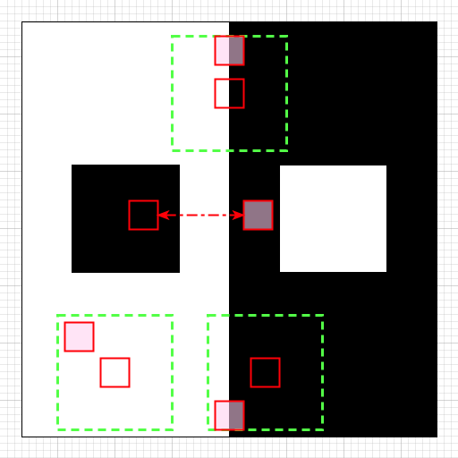
In this image, the red empty squares are patches centered on specific pixels that one wants to denoise. The dashed green squares are the corresponding learning windows. Semi-transparent red squares are examples of patches taken inside the learning windows.
The different cases are interesting:
- the topmost pixel on the vertical edge shows the interest of NL-means. Other pixels on the vertical edge will have the same black-and-white patch and will favor an output with a nice, sharp edge. Bye bye Gaussian blur!
- the black patch in the middle shows another powerful property of NL-means: if the learning window is large enough, then NL-means is able to “jump” above the white part to find another black area and provide better denoising.
- finally, the bottom patches show possible issues. For the leftmost (white) patch, only white patches will contribute to the denoising and the results should be good. For the rightmost patch (in the black area), some patches in the learning window will include a small white part. This part may not be small enough however to ensure that only correct (black) pixels will be selected.
Next episodes
In the next posts, we will see how to implement the NL-means and proceed to various experiments in order to have a good understanding of the parameters. Then, we will study several strategies to accelerate this algorithm, thus addressing its main weakness.