Linearized model of LBPs

LBP model

An LBP can be decomposed into two tiers:

• first, a real description vector, obtained by convolution-then-difference
• then the quantization (binarization) operation.

Mathematically, the real i-th component of the descriptor is computed with the formula:

$${\mathcal L}(p)_i = \langle{\mathcal G}_{x_i, \sigma_i} , p \rangle - \langle G_{x_i’, \sigma_i’} , p\rangle, $$

where ${\mathcal G}_{x_i, \sigma_i}, {\mathcal G}_{x’_i, \sigma’_i}$ are two Gaussians.

The variety of the LBP family comes from the choice of these Gaussians : they can have a fixed size but random positions (a la BRIEF), fixed sizes and positions (a la BRISK)¹… The choice in FREAK was :

1. the size of the Gaussians is fixed but depends on their position with respect to the center of the image patch (a coarser spatial resolution is used when moving away from the center)
2. the spatial layout of the Gaussians is fixed
3. the pairs of Gaussians used in the difference process are fixed, but instead of being given a priori they are produced by a learning stage.

Linearization

How can we turn an LBP into a linear operator? Well, we simply forgot or neglected the non-linear operation, i.e. we keep only the real difference vector,

OK, this is really really brutal, but there is some some intuition behind.

First, this work started as a proof-of-concept. So, the first step was logically to see if we had enough information to reconstruct the original patch from the real vector.
Second, by choosing the $\ell_1$-norm, we are not completely bound by the data term and gain some robustness against the quantization, what will be demonstrated in some experiments.

This is clearly the main limitation of the current paper, but it simplifies things greatly: if we forget about the quantization (more on this later), then we are left with an operator made of a convolution composed with a projection.

Considering the reshaping of an image patch as a column vector, applying this non-quantized operator can be obviously written as a matrix-vector operation, and we have a final problem very close to the standard space varying image deconvolution problem.

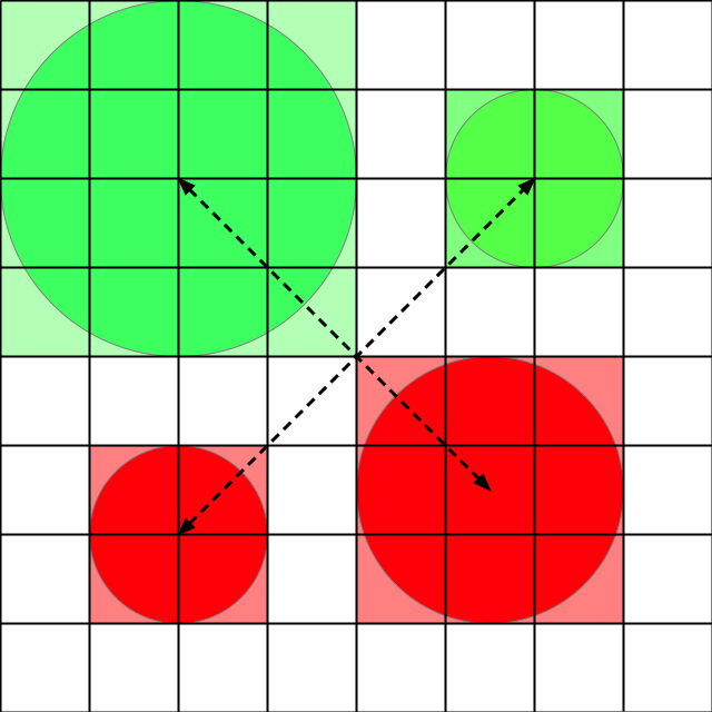
The next figures clearly show the process of forming this convoluted operator. We start with in the image domain, using for example two pairs of Gaussians:

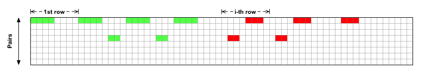
We form a row-vector from an image patch by stacking the lines of the patch in lexicographic order. Applying this same procedure to each pair of Gaussians, we naturally obtain a matrix such as the one shown in the following figure:

Moving to binary descriptors

To move to a proved and reliable 1-bit reconstruction process, our intuition is to turn to 1-bit Compressed Sensing techniques.

It is not completely clear however if this framework is fully applicable here: recall that by design FREAK is not random, because the retina-like structure was imposed and then the best pairs were selected. Hence, it is difficult to prove useful properties² like RIP of the LBP operator in this case.

Where to go next ?

Upcoming post

In the next post of the series, we will talk (at last!) about implementation tricks.

If you don’t want to miss the next posts, please subscribe to the blog ! You can also follow me on Twitter.

References for further reading

• The FREAK home page
• [DAV12] Reconstructing FREAKs: Beyond Bits: Reconstructing Images from Local Binary Descriptors, accepted at ICPR 2012
• [CLSF10] Calonder, M., Lepetit, V., Strecha, C., & Fua, P. (2010). BRIEF: Binary Robust Independent Elementary Features. Computer Vision–ECCV 2010
• [LCS11] Stefan Leutenegger, Margarita Chli and Roland Siegwart, BRISK: Binary Robust Invariant Scalable Keypoints, to appear in Proceedings of the IEEE International Conference on Computer Vision (ICCV) 2011.